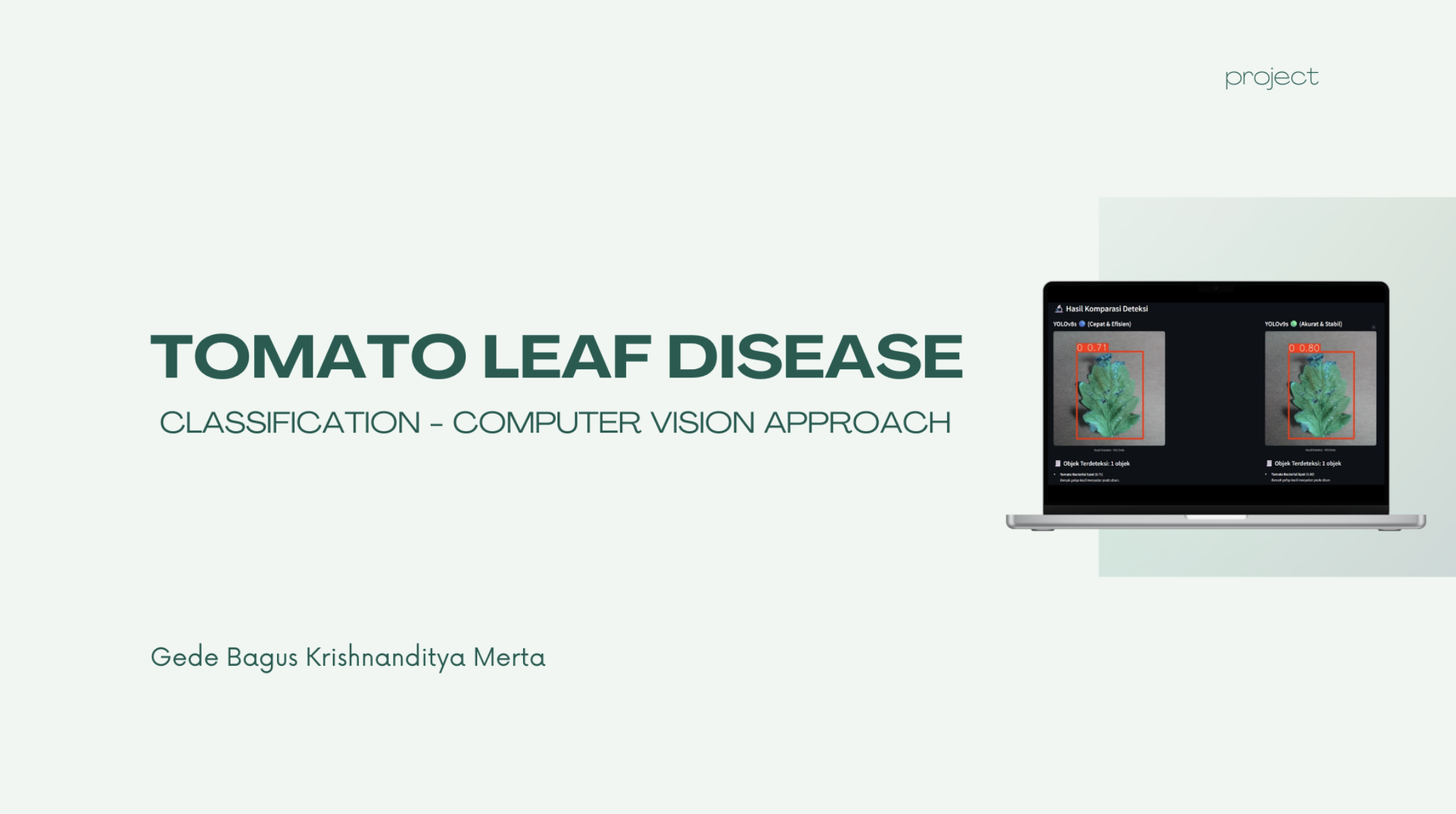
The Greenhouse Fungal Threat
In a commercial tomato greenhouse, foliar infections spread fast. What looks like a harmless brown speck on Monday morning can turn into late blight by Friday, wiping out entire rows of crops before a grower realizes the irrigation spray carried fungal spores across the aisle.
Diagnosing plant diseases by eye requires experienced agricultural inspectors. Early Blight lesions (caused by the Alternaria solani fungus) look strikingly similar to Target Spot (Corynespora cassiicola) or Septoria Leaf Spot in their early stages.
For my Computer Vision coursework at Telkom University, I wanted to build an automated diagnostic assistant and answer a practical systems question: does YOLOv9’s newer architectural complexity justify its computational overhead compared to YOLOv8 for foliar disease screening?
10,825 Raw Leaf Images (10 Disease Classes)
                    │
                    ▼
      Data Augmentation Pipeline
   (Rotation, Brightness, Mosaic Transforms)
                    │
                    ▼
         15,154 Augmented Images
                    │
                    ▼
         The Architectural Dilemma
   (Does YOLOv9's extra precision justify
    2.3x longer training times on edge devices?)
                    │
                    ▼
     Systematic Benchmark (100 Epochs)
   ├── YOLOv8s -> F1: 89.80% (77.11 mins)
   └── YOLOv9s -> F1: 92.81% (175.83 mins)
                    │
                    ▼
     Streamlit Batch Diagnostic Web App
The Ten Folia Conditions and Visual Ambiguity
The benchmark evaluated ten distinct tomato plant leaf conditions:
- Bacterial Spot (Xanthomonas bacteria)
- Early Blight (Alternaria solani fungus)
- Late Blight (Phytophthora infestans)
- Leaf Mold (Passalora fulva)
- Septoria Leaf Spot (Septoria lycopersici)
- Spider Mites (Tetranychus urticae)
- Target Spot (Corynespora cassiicola)
- Tomato Yellow Leaf Curl Virus (whitefly-transmitted)
- Tomato Mosaic Virus
- Healthy leaves with no pathogenic markings
The raw dataset contained 10,825 images. Because camera angles and greenhouse daylight vary widely, I expanded the training set to 15,154 images using horizontal flips, random rotations, brightness variations, and mosaic augmentations.
Mosaic augmentation combines four randomly cropped training images into one tile, forcing the detector to learn disease patterns at different zoom scales and near bounding box borders.
Does YOLOv9’s Programmable Gradient Information make a measurable difference on small foliar lesions?
Training and Benchmarking the Two Architectures
Using the Ultralytics framework and OpenCV, I trained both yolov8s and yolov9s across 100 epochs on identical 640x640 input resolutions:
from ultralytics import YOLO

# Training script for both candidate backbones
model_v8 = YOLO('yolov8s.yaml')
model_v8.train(data='tomato.yaml', epochs=100, imgsz=640, device=0)

model_v9 = YOLO('yolov9s.yaml')
model_v9.train(data='tomato.yaml', epochs=100, imgsz=640, device=0)
YOLOv9 introduces Programmable Gradient Information (PGI) and a Generalized Efficient Layer Aggregation Network (GELAN) architecture, designed to prevent information loss as features travel through deep convolutional layers.
Evaluating both models on a dedicated holdout test set yielded a clear performance gap:
| Model Architecture | Precision | Recall | F1-Score | Training Wall Time |
|---|---|---|---|---|
| YOLOv8s | 89.50% | 90.10% | 89.80% | 77.11 minutes |
| YOLOv9s | 92.74% | 92.88% | 92.81% | 175.83 minutes |
YOLOv9s achieved an F1-score gain of +3.01% (92.81% versus 89.80%).
Examining the detections showed that YOLOv9’s advantage was strongest on tiny, clustered lesions like Septoria Leaf Spot and early Spider Mite stippling. Where YOLOv8s occasionally merged adjacent micro-spots into one blurred box or missed faint spots near leaf veins, YOLOv9’s gradient preservation helped it resolve discrete lesion borders.
However, that 3% precision gain came at a steep cost: training took 175.83 minutes (nearly three hours), representing a 2.3x increase in compute time over YOLOv8s’s 77.11 minutes.
Deployment Trade-offs in Agriculture
To allow practical testing, I connected the pipeline to an interactive Streamlit web application with OpenCV image normalization:
Farmer Uploads Photo or Connects Camera
                    │
                    ▼
      OpenCV Image Normalization
      (BGR to RGB, Resizing to 640x640)
                    │
                    ▼
          Tuned YOLO Inference
                    │
                    ▼
   Annotated Output with Bounding Boxes,
   Disease Class Labels, & Confidence Scores
The application accepts single leaf snapshots or batch folder uploads from field surveys, rendering labeled bounding boxes and exporting a CSV summary of detected disease distributions.
The comparative benchmark presents a clear trade-off:
- If you are building a central laboratory web portal running on high-end cloud GPUs where every fraction of a percent counts for quarantine decisions, YOLOv9s is the superior engine.
- If you are deploying edge inference on a low-power single-board computer mounted inside a greenhouse sprinkler rig, YOLOv8s is far more practical. It delivers 89.8% F1 while training in half the time and maintaining lower inference latency.
What I Learned
Benchmarking YOLOv8 against YOLOv9 reminded me that benchmark leadership is contextual.
It is easy to look at an ML leaderboard and declare the newest model the automatic winner. But in agricultural computing, hardware constraints, electrical budgets, and training iteration speed matter just as much as raw mean Average Precision.
Understanding exactly what you buy with that extra computational cost (in our case, better sensitivity on tiny Septoria spots in exchange for 2.3x longer training runs) is the difference between academic theory and practical system design.